Plot evolution of diversification rates in relation to trait values over time
Source:R/plot_rates_through_time.R
plot_rates_through_time.RdPlot the evolution of diversification rates in relation to trait values
extracted for multiple time_steps with run_deepSTRAPP_over_time().
Rates are averaged across branches at each time step (i.e., focal_time).
For continuous data, branches are grouped by ranges of trait values defined by
quantile_ranges.For categorical data, branches are grouped by trait states.
For biogeographic data, branches are grouped by ranges.
Usage
plot_rates_through_time(
  deepSTRAPP_outputs,
  rate_type = "net_diversification",
  quantile_ranges = c(0, 0.25, 0.5, 0.75, 1),
  select_trait_levels = "all",
  time_range = NULL,
  color_scale = NULL,
  colors_per_levels = NULL,
  plot_CI = FALSE,
  CI_type = "fuzzy",
  CI_quantiles = 0.95,
  display_plot = TRUE,
  PDF_file_path = NULL,
  return_mean_data_per_samples_df = FALSE,
  return_median_data_across_samples_df = FALSE
)
Arguments
- deepSTRAPP_outputs
List of elements generated with
run_deepSTRAPP_over_time(), that summarize the results of multiple STRAPP tests across$time_steps. The list needs to include two data.frame:$trait_data_df_over_timeand$diversification_data_df_over_timeby settingextract_trait_data_melted_df = TRUEandextract_diversification_data_melted_df = TRUE.- rate_type
A character string specifying the type of diversification rates to use. Must be one of 'speciation', 'extinction' or 'net_diversification' (default). Even if the
deepSTRAPP_outputsobject was generated withrun_deepSTRAPP_over_time()for testing another type of rates, the$trait_data_df_over_timeand$diversification_data_df_over_timedata frames will contain data for all types of rates.- quantile_ranges
Vector of numerical. Only for continuous trait data. Quantiles used as thresholds to group branches by trait values. It must start with 0 and finish with 1. Default is
c(0, 0.25, 0.5, 0.75, 1.0)which produces four balanced quantile groups.- select_trait_levels
(Vector of) character string. Only for categorical and biogeographic trait data. To provide a list of a subset of states/ranges to plot. Names must match the ones found in
deepSTRAPP_outputs$trait_data_df_over_time$trait_value. Default isallwhich means all states/ranges will be plotted.- time_range
Vector of two numerical values. Time boundaries used for the plot. If
NULL(the default), the range of data provided indeepSTRAPP_outputswill be used.- color_scale
Vector of character string. List of colors to use to build the color scale with
grDevices::colorRampPalette()to display the quantile groups used to discretize the continuous trait data. From lowest values to highest values. Only for continuous data. Default =NULLwill use the 'Spectral' color palette inRColorBrewer::brewer.pal().- colors_per_levels
Named character string. To set the colors to use to plot rates of each state/range. Names = states/ranges; values = colors. If
NULL(default), the default ggplot2 color palette (scales::hue_pal()) will be used. Only for categorical and biogeographic data.- plot_CI
Logical. Whether to plot a confidence interval (CI) based on the distribution of rates found in posterior samples. Default is
FALSE.- CI_type
Character string. To select the type of confidence interval (CI) to plot.
fuzzy(default): to overlay the evolution of rates found in all posterior samples with high transparency levels.quantiles_rect: to add a polygon encompassing a proportion of the rate values found in posterior samples. This proportion is defined withCI_quantiles.
- CI_quantiles
Numerical. Proportion of rate values across posterior samples encompassed by the confidence interval. Only if
CI_type = "quantiles_rect". Default is0.95.- display_plot
Logical. Whether to display the plot generated in the R console. Default is
TRUE.- PDF_file_path
Character string. If provided, the plot will be saved in a PDF file following the path provided here. The path must end with ".pdf".
- return_mean_data_per_samples_df
Logical. Whether to include in the output the data.frame of mean rates per trait values computed for each posterior sample at each time-step (aggregated across groups of branches based on trait data). This is used to draw the confidence interval. Default is
FALSE.- return_median_data_across_samples_df
Logical. Whether to include in the output the data.frame of median rates per trait values across posterior samples computed for at each time-step (aggregated across groups of branches based on trait data AND posterior samples). This is used to draw the lines on the plot. Default is
FALSE.
Value
The function returns a list with at least one element.
rates_TT_ggplotAn object of classesggandggplot. This is a ggplot that can be displayed on the console withprint(output$rates_TT_ggplot). It corresponds to the plot being displayed on the console when the function is run, ifdisplay_plot = TRUE, and can be further modify for aesthetics using the ggplot2 grammar.
Optional summary data frames:
mean_data_per_samples_dfA data.frame with four columns providing the$mean_ratesobserved along branches with a similar$trait_value(if categorical or biogeographic) or falling into the same$quantile_ranges. Data are extracted for each posterior sample ($BAMM_sample_ID) at each time-step (i.e.,$focal_time). This is used to draw the confidence interval. Included ifreturn_mean_data_per_samples_df = TRUE.$median_data_across_samples_dfA data.frame with three columns providing the$median_ratesobserved across all posterior samples in$mean_data_per_samples_df. This is used to draw the lines on the plot. Included ifreturn_median_data_across_samples_df = TRUE.
If a PDF_file_path is provided, the function will also generate a PDF file of the plot.
See also
For a guided tutorial, see this vignette: vignette("plot_rates_through_time", package = "deepSTRAPP")
Examples
# ------ Example 1: Plot rates through time for continuous data ------ #
## Load results of run_deepSTRAPP_over_time()
data(Ponerinae_deepSTRAPP_cont_old_calib_0_40, package = "deepSTRAPP")
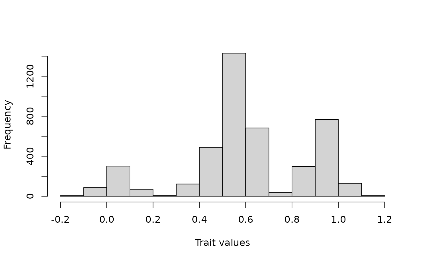
# Visualize trait data
hist(Ponerinae_deepSTRAPP_cont_old_calib_0_40$trait_data_df_over_time$trait_value,
xlab = "Trait values", main = NULL)
 # Generate plot
plotTT_continuous <- plot_rates_through_time(
deepSTRAPP_outputs = Ponerinae_deepSTRAPP_cont_old_calib_0_40,
quantile_ranges = c(0, 0.25, 0.5, 0.75, 1.0),
time_range = c(0, 50), # Control range of the X-axis
# color_scale = c("limegreen", "red"),
plot_CI = TRUE,
CI_type = "quantiles_rect",
CI_quantiles = 0.9,
display_plot = FALSE,
# PDF_file_path = "./plotTT_continuous.pdf",
return_mean_data_per_samples_df = TRUE,
return_median_data_across_samples_df = TRUE)
# Explore output
# str(plotTT_continuous, max.level = 1)
# Plot
print(plotTT_continuous$rates_TT_ggplot)
# Generate plot
plotTT_continuous <- plot_rates_through_time(
deepSTRAPP_outputs = Ponerinae_deepSTRAPP_cont_old_calib_0_40,
quantile_ranges = c(0, 0.25, 0.5, 0.75, 1.0),
time_range = c(0, 50), # Control range of the X-axis
# color_scale = c("limegreen", "red"),
plot_CI = TRUE,
CI_type = "quantiles_rect",
CI_quantiles = 0.9,
display_plot = FALSE,
# PDF_file_path = "./plotTT_continuous.pdf",
return_mean_data_per_samples_df = TRUE,
return_median_data_across_samples_df = TRUE)
# Explore output
# str(plotTT_continuous, max.level = 1)
# Plot
print(plotTT_continuous$rates_TT_ggplot)
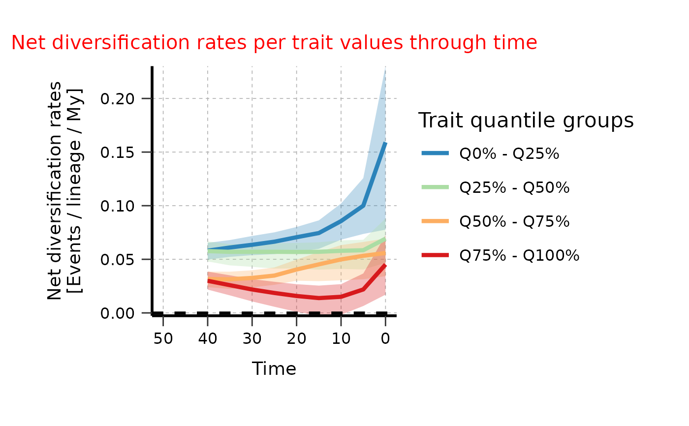
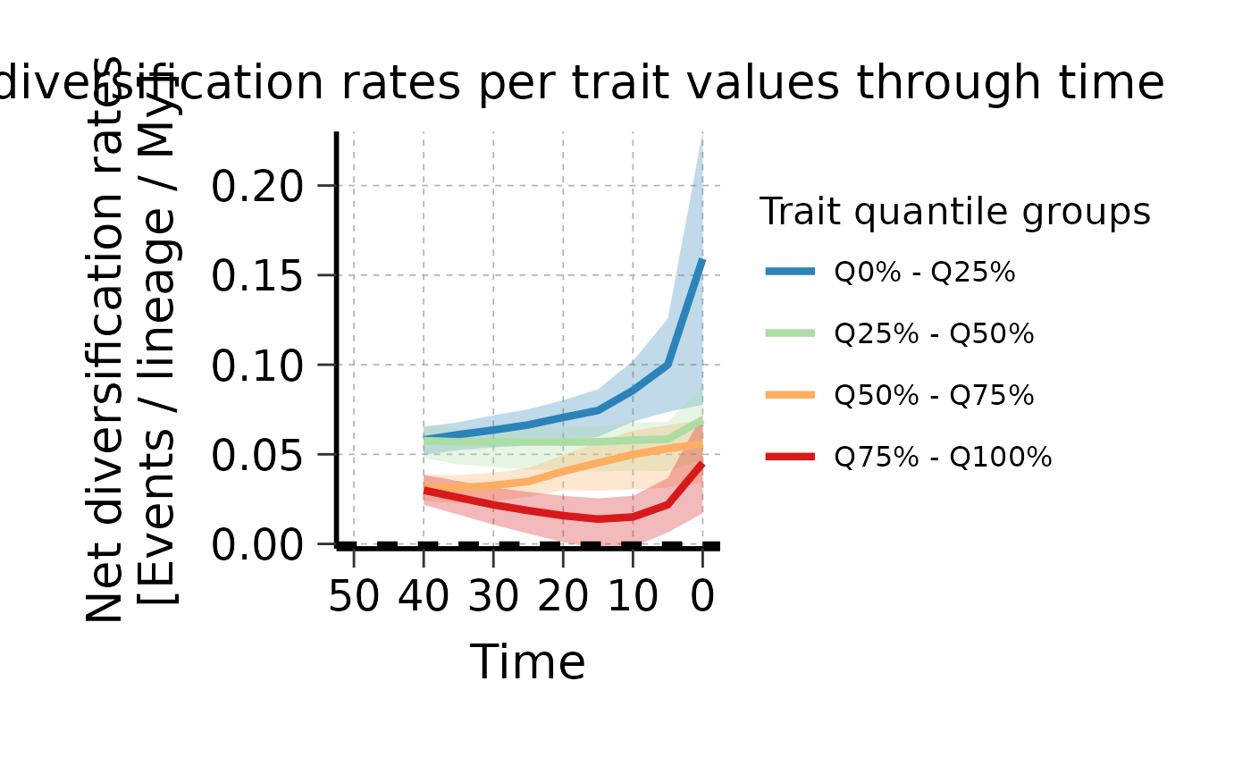 # Adjust aesthetics of plot a posteriori
plotTT_continuous_adj <- plotTT_continuous$rates_TT_ggplot +
ggplot2::theme(
plot.title = ggplot2::element_text(color = "red", size = 15),
axis.title = ggplot2::element_text(size = 14),
axis.text = ggplot2::element_text(size = 12))
# Plot again
print(plotTT_continuous_adj)
# Adjust aesthetics of plot a posteriori
plotTT_continuous_adj <- plotTT_continuous$rates_TT_ggplot +
ggplot2::theme(
plot.title = ggplot2::element_text(color = "red", size = 15),
axis.title = ggplot2::element_text(size = 14),
axis.text = ggplot2::element_text(size = 12))
# Plot again
print(plotTT_continuous_adj)
 # ------ Example 2: Plot rates through time for categorical data ------ #
## Load results of run_deepSTRAPP_over_time()
data(Ponerinae_deepSTRAPP_cat_3lvl_old_calib_0_40, package = "deepSTRAPP")
# Explore trait data
table(Ponerinae_deepSTRAPP_cat_3lvl_old_calib_0_40$trait_data_df_over_time$trait_value)
#>
#> arboreal subterranean terricolous
#> 1063 2883 489
# Set colors to use
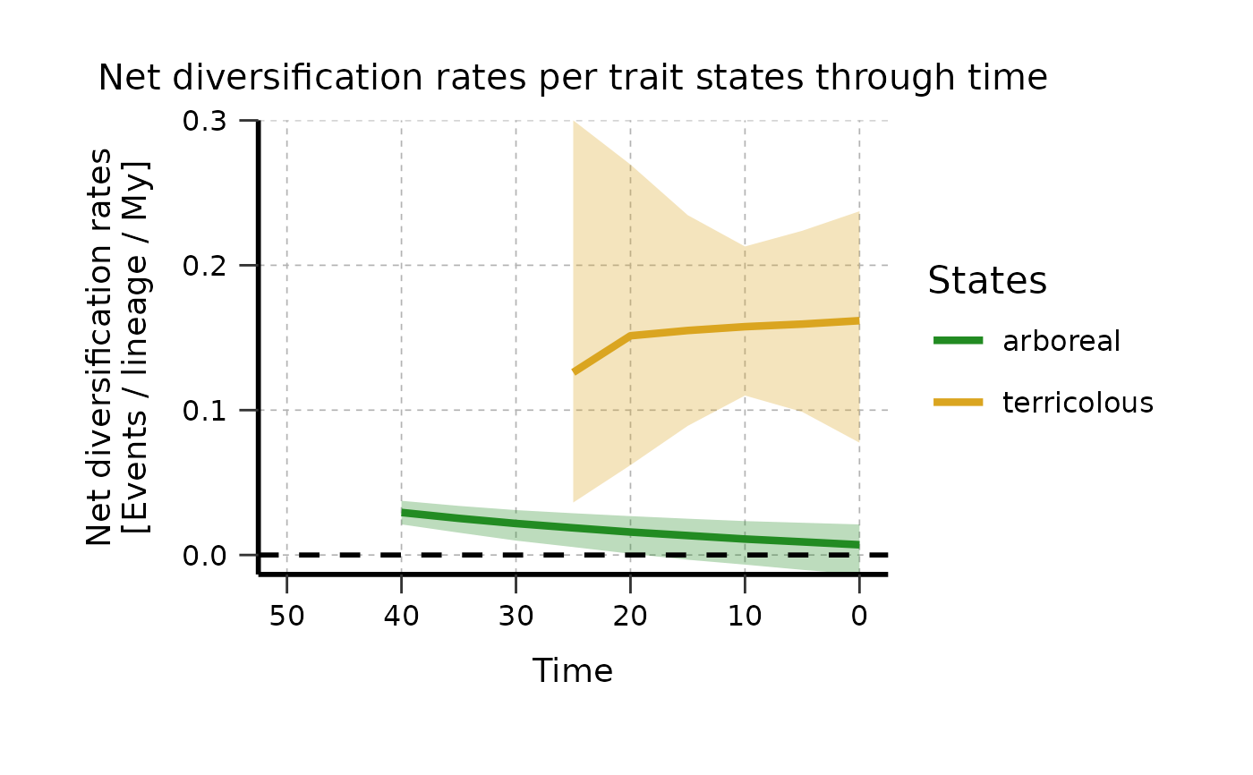
colors_per_states <- c("forestgreen", "sienna", "goldenrod")
names(colors_per_states) <- c("arboreal", "subterranean", "terricolous")
plotTT_categorical <- plot_rates_through_time(
deepSTRAPP_outputs = Ponerinae_deepSTRAPP_cat_3lvl_old_calib_0_40,
select_trait_levels = c("arboreal", "terricolous"),
time_range = c(0, 50),
colors_per_levels = colors_per_states,
plot_CI = TRUE,
CI_type = "quantiles_rect",
CI_quantiles = 0.9,
display_plot = FALSE,
# PDF_file_path = "./plotTT_categorical.pdf",
return_mean_data_per_samples_df = TRUE,
return_median_data_across_samples_df = TRUE)
# Explore output
# str(plotTT_categorical, max.level = 1)
# Adjust aesthetics of plot a posteriori
plotTT_categorical_adj <- plotTT_categorical$rates_TT_ggplot +
ggplot2::theme(
plot.title = ggplot2::element_text(size = 15),
axis.title = ggplot2::element_text(size = 14),
axis.text = ggplot2::element_text(size = 12))
print(plotTT_categorical_adj)
# ------ Example 2: Plot rates through time for categorical data ------ #
## Load results of run_deepSTRAPP_over_time()
data(Ponerinae_deepSTRAPP_cat_3lvl_old_calib_0_40, package = "deepSTRAPP")
# Explore trait data
table(Ponerinae_deepSTRAPP_cat_3lvl_old_calib_0_40$trait_data_df_over_time$trait_value)
#>
#> arboreal subterranean terricolous
#> 1063 2883 489
# Set colors to use
colors_per_states <- c("forestgreen", "sienna", "goldenrod")
names(colors_per_states) <- c("arboreal", "subterranean", "terricolous")
plotTT_categorical <- plot_rates_through_time(
deepSTRAPP_outputs = Ponerinae_deepSTRAPP_cat_3lvl_old_calib_0_40,
select_trait_levels = c("arboreal", "terricolous"),
time_range = c(0, 50),
colors_per_levels = colors_per_states,
plot_CI = TRUE,
CI_type = "quantiles_rect",
CI_quantiles = 0.9,
display_plot = FALSE,
# PDF_file_path = "./plotTT_categorical.pdf",
return_mean_data_per_samples_df = TRUE,
return_median_data_across_samples_df = TRUE)
# Explore output
# str(plotTT_categorical, max.level = 1)
# Adjust aesthetics of plot a posteriori
plotTT_categorical_adj <- plotTT_categorical$rates_TT_ggplot +
ggplot2::theme(
plot.title = ggplot2::element_text(size = 15),
axis.title = ggplot2::element_text(size = 14),
axis.text = ggplot2::element_text(size = 12))
print(plotTT_categorical_adj)
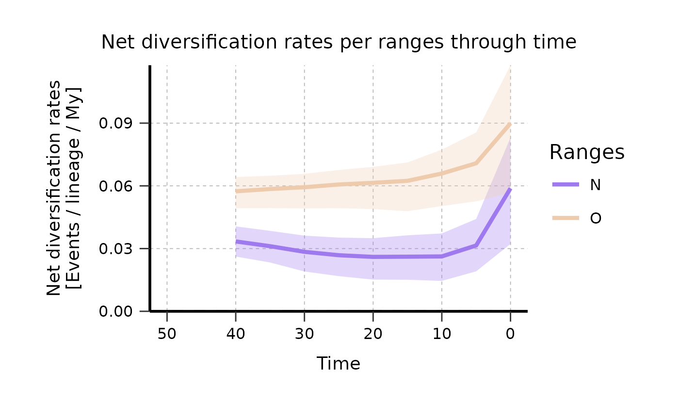
 # ------ Example 3: Plot rates through time for biogeographic data ------ #
## Load results of run_deepSTRAPP_over_time()
data(Ponerinae_deepSTRAPP_biogeo_old_calib_0_40, package = "deepSTRAPP")
# Explore range data
table(Ponerinae_deepSTRAPP_biogeo_old_calib_0_40$trait_data_df_over_time$trait_value)
#>
#> N O
#> 1587 2848
# Set colors to use
colors_per_ranges <- c("mediumpurple2", "peachpuff2")
names(colors_per_ranges) <- c("N", "O")
plotTT_biogeographic <- plot_rates_through_time(
deepSTRAPP_outputs = Ponerinae_deepSTRAPP_biogeo_old_calib_0_40,
select_trait_levels = "all",
time_range = c(0, 50),
colors_per_levels = colors_per_ranges,
plot_CI = TRUE,
CI_type = "quantiles_rect",
CI_quantiles = 0.9,
display_plot = FALSE,
# PDF_file_path = "./plotTT_biogeographic.pdf",
return_mean_data_per_samples_df = TRUE,
return_median_data_across_samples_df = TRUE)
# Explore output
# str(plotTT_biogeographic, max.level = 1)
# Adjust aesthetics of plot a posteriori
plotTT_biogeographic_adj <- plotTT_biogeographic$rates_TT_ggplot +
ggplot2::theme(
plot.title = ggplot2::element_text(size = 15),
axis.title = ggplot2::element_text(size = 14),
axis.text = ggplot2::element_text(size = 12))
print(plotTT_biogeographic_adj)
# ------ Example 3: Plot rates through time for biogeographic data ------ #
## Load results of run_deepSTRAPP_over_time()
data(Ponerinae_deepSTRAPP_biogeo_old_calib_0_40, package = "deepSTRAPP")
# Explore range data
table(Ponerinae_deepSTRAPP_biogeo_old_calib_0_40$trait_data_df_over_time$trait_value)
#>
#> N O
#> 1587 2848
# Set colors to use
colors_per_ranges <- c("mediumpurple2", "peachpuff2")
names(colors_per_ranges) <- c("N", "O")
plotTT_biogeographic <- plot_rates_through_time(
deepSTRAPP_outputs = Ponerinae_deepSTRAPP_biogeo_old_calib_0_40,
select_trait_levels = "all",
time_range = c(0, 50),
colors_per_levels = colors_per_ranges,
plot_CI = TRUE,
CI_type = "quantiles_rect",
CI_quantiles = 0.9,
display_plot = FALSE,
# PDF_file_path = "./plotTT_biogeographic.pdf",
return_mean_data_per_samples_df = TRUE,
return_median_data_across_samples_df = TRUE)
# Explore output
# str(plotTT_biogeographic, max.level = 1)
# Adjust aesthetics of plot a posteriori
plotTT_biogeographic_adj <- plotTT_biogeographic$rates_TT_ggplot +
ggplot2::theme(
plot.title = ggplot2::element_text(size = 15),
axis.title = ggplot2::element_text(size = 14),
axis.text = ggplot2::element_text(size = 12))
print(plotTT_biogeographic_adj)