deepSTRAPP: Continuous trait data

This is a simple example that shows how deepSTRAPP can be used to test for correlations between a continuous trait and diversification rates along evolutionary times. It presents the main functions in a typical deepSTRAPP workflow.

For an example with binary data (2 levels), please see the example in the Main tutorial: vignette("main_tutorial").

For an example with biogeographic data, see this vignette: vignette("deepSTRAPP_biogeographic_data").

Please note that the trait data and phylogeny calibration used in this example are NOT valid biological data. They were modified in order to provide results illustrating the usefulness of deepSTRAPP.

# ------ Step 0: Load data ------ #

## Load trait df
data("Ponerinae_trait_tip_data", package = "deepSTRAPP")

dim(Ponerinae_trait_tip_data)
View(Ponerinae_trait_tip_data)

# Extract continuous trait data as a named vector
Ponerinae_cont_tip_data <- setNames(object = Ponerinae_trait_tip_data$fake_cont_tip_data,
                                    nm = Ponerinae_trait_tip_data$Taxa)

# This not valid biological data. For the sake of this example, we will assume this is size data.

# Select a color scheme from lowest to highest values (i.e., smallest to largest ants)
color_scale = c("darkgreen", "limegreen", "orange", "red")

## Load phylogeny with old time-calibration
data("Ponerinae_tree_old_calib", package = "deepSTRAPP")

plot(Ponerinae_tree_old_calib)
ape::Ntip(Ponerinae_tree_old_calib) == length(Ponerinae_cont_tip_data)

## Check that trait data and phylogeny are named and ordered similarly
all(names(Ponerinae_cont_tip_data) == Ponerinae_tree_old_calib$tip.label)


## Inputs needed for Step 1 are the tip_data (Ponerinae_cont_tip_data) and the phylogeny
# (Ponerinae_tree_old_calib), and optionally, a color scheme (color_scale).

# ------ Step 1: Prepare trait data ------ #

## Goal: Map trait evolution on the time-calibrated phylogeny

# 1.1/ Fit evolutionary models to trait data using Maximum Likelihood.
# 1.2/ Select the best fitting model comparing AICc.
# 1.3/ Infer ancestral characters estimates (ACE) at nodes.
# 1.4/ Infer ancestral states along branches using interpolation to produce a `contMap`.

library(deepSTRAPP)

# All these actions are performed by a single function: deepSTRAPP::prepare_trait_data()
?deepSTRAPP::prepare_trait_data()

# Run prepare_trait_data with default options
# For continuous trait, a BM model is assumed by default.
Ponerinae_trait_object <- prepare_trait_data(tip_data = Ponerinae_cont_tip_data,
                                             trait_data_type = "continuous",
                                             phylo = Ponerinae_tree_old_calib,
                                             seed = 1234) # Set seed for reproducibility

# Explore output
str(Ponerinae_trait_object, 1)

# Extract the contMap representing continuous trait evolution on the phylogeny
Ponerinae_contMap <- Ponerinae_trait_object$contMap
plot_contMap(Ponerinae_contMap)

# Extract the Ancestral Character Estimates (ACE) = trait values at nodes
Ponerinae_ACE <- Ponerinae_trait_object$ace
head(Ponerinae_ACE)

## Inputs needed for Step 2 are the contMap, and optionally, the tip_data (Ponerinae_cont_tip_data),
# and the ACE (Ponerinae_ACE)

# ------ Step 2: Prepare diversification data ------ #

## Goal: Map evolution of diversification rates and regime shifts on the time-calibrated phylogeny

# Run a BAMM (Bayesian Analysis of Macroevolutionary Mixtures)

# You need the BAMM C++ program installed in your machine to run this step.
# See the BAMM website: http://bamm-project.org/ and the companion R package [BAMMtools].

# 2.1/ Set BAMM - Record BAMM settings and generate all input files needed for BAMM.
# 2.2/ Run BAMM - Run BAMM and move output files in dedicated directory.
# 2.3/ Evaluate BAMM - Produce evaluation plots and ESS data.
# 2.4/ Import BAMM outputs - Load `BAMM_object` in R and subset posterior samples.
# 2.5/ Clean BAMM files - Remove files generated during the BAMM run.

# All these actions are performed by a single function: deepSTRAPP::prepare_diversification_data()
?deepSTRAPP::prepare_diversification_data()

# Run BAMM workflow with deepSTRAPP
## This step is time-consuming. You can skip it and load directly the result if needed
Ponerinae_BAMM_object_old_calib <- prepare_diversification_data(
   BAMM_install_directory_path = "./software/bamm-2.5.0/", # To adjust to your own path to BAMM
   phylo = Ponerinae_tree_old_calib,
   prefix_for_files = "Ponerinae",
   seed = 1234, # Set seed for reproducibility
   numberOfGenerations = 10^7 # Set high for optimal run, but will take a long time
)

# Load directly the result
data(Ponerinae_BAMM_object_old_calib)

# Explore output
str(Ponerinae_BAMM_object_old_calib, 1)
# Record the regime shift events and macroevolutionary regimes parameters across posterior samples
str(Ponerinae_BAMM_object_old_calib$eventData, 1) 
# Mean speciation rates at tips aggregated across all posterior samples
head(Ponerinae_BAMM_object_old_calib$meanTipLambda) 
# Mean extinction rates at tips aggregated across all posterior samples
head(Ponerinae_BAMM_object_old_calib$meanTipMu) 

# Plot mean net diversification rates and regime shifts on the phylogeny
plot_BAMM_rates(Ponerinae_BAMM_object_old_calib,
                labels = FALSE, legend = TRUE)

## Input needed for Step 3 is the BAMM_object (Ponerinae_BAMM_object)

# ------ Step 3: Run a deepSTRAPP workflow ------ #

## Goal: Extract traits, diversification rates and regimes at a given time in the past
# to test for differences with a STRAPP test

# 3.1/ Extract trait data at a given time in the past ('focal_time')
# 3.2/ Extract diversification rates and regimes at a given time in the past ('focal_time')
# 3.3/ Compute STRAPP test
# 3.4/ Repeat previous actions for many timesteps along evolutionary time

# All these actions are performed by a single function:
#  For a single 'focal_time': deepSTRAPP::run_deepSTRAPP_for_focal_time()
#  For multiple 'time_steps': deepSTRAPP::run_deepSTRAPP_over_time()
?deepSTRAPP::run_deepSTRAPP_for_focal_time()
?deepSTRAPP::run_deepSTRAPP_over_time()

## Set for time steps of 5 My. Will generate deepSTRAPP workflows for 0 to 40 Mya.
# nb_time_steps <- 5
time_step_duration <- 5
time_range <- c(0, 40)

# Run deepSTRAPP on net diversification rates
## This step is time-consuming. You can skip it and load directly the result if needed
Ponerinae_deepSTRAPP_cont_old_calib_0_40 <- run_deepSTRAPP_over_time(
    contMap = Ponerinae_contMap,
    ace = Ponerinae_ACE,
    tip_data = Ponerinae_cont_tip_data,
    trait_data_type = "continuous",
    BAMM_object = Ponerinae_BAMM_object_old_calib,
    # nb_time_steps = nb_time_steps,
    time_range = time_range,
    time_step_duration = time_step_duration,
    seed = 1234, # Set seed for reproducibility
    # Needed to obtain STRAPP stats and plot evaluation histograms (See 4.2)
    return_perm_data = TRUE, 
    # Needed to get trait data and plot rates through time (See 4.3)
    extract_trait_data_melted_df = TRUE, 
    # Needed to get diversification data and plot rates through time (See 4.3)
    extract_diversification_data_melted_df = TRUE, 
    # Needed to obtain STRAPP stats and plot evaluation histograms (See 4.2)
    return_STRAPP_results = TRUE, 
    # Needed to plot updated contMaps (See 4.4)
    return_updated_trait_data_with_Map = TRUE, 
    # Needed to map diversification rates on updated phylogenies (See 4.5)
    return_updated_BAMM_object = TRUE, 
    verbose = TRUE,
    verbose_extended = TRUE)

# Load the deepSTRAPP output summarizing results for 0 to 40 My
data(Ponerinae_deepSTRAPP_cont_old_calib_0_40, package = "deepSTRAPP")

## Explore output
str(Ponerinae_deepSTRAPP_cont_old_calib_0_40, max.level = 1)

# See next step for how to generate plots from those outputs

# Display test summary
# Can be passed down to [deepSTRAPP::plot_STRAPP_pvalues_over_time()] to generate a plot
# showing the evolution of the test results across time
Ponerinae_deepSTRAPP_cont_old_calib_0_40$pvalues_summary_df

# Access STRAPP test results
# Can be passed down to [deepSTRAPP::plot_histograms_STRAPP_tests_over_time()] to generate plot
# showing the null distribution of the test statistics
str(Ponerinae_deepSTRAPP_cont_old_calib_0_40$STRAPP_results, max.level = 2)

# Access trait data in a melted data.frame
head(Ponerinae_deepSTRAPP_cont_old_calib_0_40$trait_data_df_over_time)
# Access the diversification data in a melted data.frame
head(Ponerinae_deepSTRAPP_cont_old_calib_0_40$diversification_data_df_over_time)
# Both can be passed down to [deepSTRAPP::plot_rates_through_time()] to generate a plot
# showing the evolution of diversification rates though time in relation to trait values

# Access updated contMaps for each focal time
# Can be used to plot contMap with branch cut-off at focal time with [deepSTRAPP::plot_contMap()]
str(Ponerinae_deepSTRAPP_cont_old_calib_0_40$updated_trait_data_with_Map_over_time, max.level = 2)

# Access updated BAMM_object for each focal time
# Can be used to map rates and regime shifts on phylogeny with branch cut-off 
# at focal time with [deepSTRAPP::plot_BAMM_rates()]
str(Ponerinae_deepSTRAPP_cont_old_calib_0_40$updated_BAMM_objects_over_time, max.level = 2)

## Input needed for Step 4 is the deepSTRAPP object (Ponerinae_deepSTRAPP_cont_old_calib_0_40)

# ------ Step 4: Plot results ------ #

## Goal: Summarize the outputs in meaningful plots

# 4.1/ Plot evolution of STRAPP tests p-values through time
# 4.2/ Plot histogram of STRAPP test stats
# 4.3/ Plot evolution of rates through time in relation to trait values
# 4.4/ Plot rates vs. trait values across branches for a given 'focal_time'
# 4.5/ Plot updated densityMaps mapping trait evolution for a given 'focal_time'
# 4.6/ Plot updated diversification rates and regimes for a given 'focal_time'
# 4.7/ Combine 4.5 and 4.6 to plot both mapped phylogenies with trait evolution (4.5)
#      and diversification rates and regimes (4.6).

# Each plot is achieved through a dedicated function

# Load the deepSTRAPP output summarizing results for 0 to 40 My
data(Ponerinae_deepSTRAPP_cont_old_calib_0_40, package = "deepSTRAPP")

### 4.1/ Plot evolution of STRAPP tests p-values through time ####

# ?deepSTRAPP::plot_STRAPP_pvalues_over_time()

## Plot results of Spearman's tests over time
deepSTRAPP::plot_STRAPP_pvalues_over_time(
   deepSTRAPP_outputs = Ponerinae_deepSTRAPP_cont_old_calib_0_40)

# This is the main output of deepSTRAPP. It shows the evolution of the significance
# of the STRAPP tests over time.
# This example highlights the importance of deepSTRAPP as the significance of STRAPP tests
# change over time. 
# Correlation between trait values and net diversification rates are not significant in the present
# (assuming a significant threshold of alpha = 0.05).
# Meanwhile, correlations were significant in the past between 5 My to 25 My (the green area).
# This result supports the idea that differences in biodiversity in relation to trait values
# (e.g., ant size) can be explained by correlations between rates and net diversification rates
# that occurred in the past. Without use of deepSTRAPP, this conclusion would not have been supported
# by current diversification rates alone.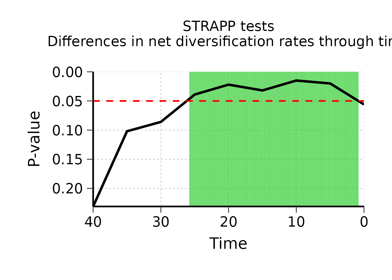

### 4.2/ Plot histogram of STRAPP test stats ####

# Plot an histogram of the distribution of the test statistics used to assess
# the significance of STRAPP tests
  #  For a single 'focal_time': deepSTRAPP::plot_histogram_STRAPP_test_for_focal_time()
  #  For multiple 'time_steps': deepSTRAPP::plot_histograms_STRAPP_tests_over_time()

# ?deepSTRAPP::plot_histogram_STRAPP_test_for_focal_time
# ?deepSTRAPP::plot_histograms_STRAPP_tests_over_time

## These functions are used to provide visual illustration of the results of each STRAPP test. 
# They can be used to complement the provision of the statistical results summarized in Step 3.

# Display the time-steps
Ponerinae_deepSTRAPP_cont_old_calib_0_40$time_steps

# Plot the histogram of test stats for time-step n°5 = 20 My
plot_histogram_STRAPP_test_for_focal_time(
   deepSTRAPP_outputs = Ponerinae_deepSTRAPP_cont_old_calib_0_40,
   focal_time = 20)

# The black line represents the expected value under the null hypothesis H0 => Δ abs(Spearman rho stat) = 0.
# The histogram shows the distribution of the test statistics as observed
# across the 1000 posterior samples from BAMM.
# The red line represents the significance threshold for which 95% of the observed data
# exhibited a higher value than expected.
# Since this red line is above the null expectation (quantile 5% = 0.036), 
# the test is significant for a value of alpha = 0.05.
# Therefore, ant size was significantly correlated with net diversification rates 20 Mya.
# Since we performed a two-tailed test (default), we do not know the direction of this correlation (yet).

# Plot the histograms of test stats for all time-steps
plot_histograms_STRAPP_tests_over_time(
   deepSTRAPP_outputs = Ponerinae_deepSTRAPP_cont_old_calib_0_40)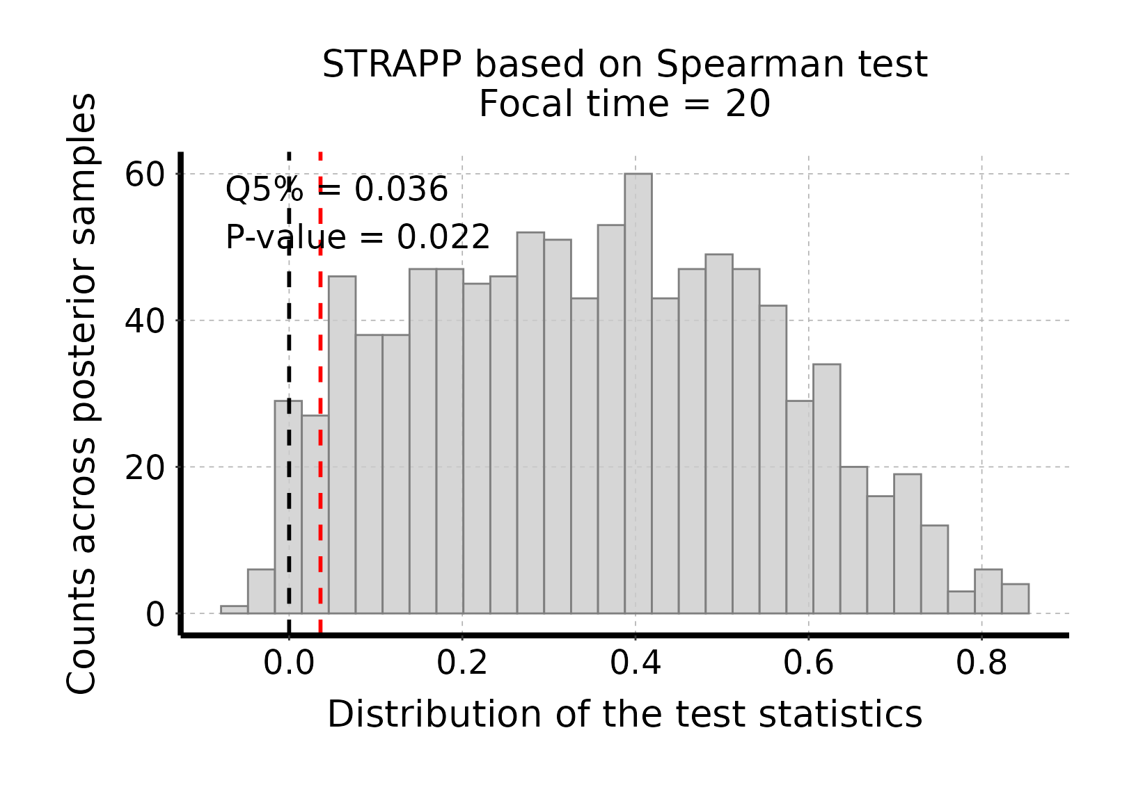

### 4.3/ Plot evolution of rates through time ~ trait data ####

# ?deepSTRAPP::plot_rates_through_time()

# Generate ggplot
plot_rates_through_time(deepSTRAPP_outputs = Ponerinae_deepSTRAPP_cont_old_calib_0_40,
                        plot_CI = TRUE)

# This plot helps to visualize how correlations between trait values and rates evolved over time.
# Here, we observe a "negative" correlation as ants in the lowest quartile of trait values (in blue)
# display the highest net diversification rates over time, while ants in the highest quartile
# of trait values (in red) display the lowest net diversification rates over time.
# However, in the present, we recorded an increase in diversification rates that blurred 
# these differences and led to a non-significant STRAPP test when comparing current rates.
# This plot, alongside results of deepSTRAPP, supports the Diversification Rate Hypothesis
# in showing how ant lineages with low trait values (e.g., small size) may have accumulated faster
# than ant lineages with high trait value (e.g., large size), especially between 5 to 25 My.

# N.B.: The increase of diversification rates recorded in the present may largely be artifactual,
# due to the fact some lineages in the present will go extinct in the future,
# but have not yet been recorded as such. 
# This bias is named the "pull of the present", and can impair evaluation of 
# the Diversification Rate Hypothesis based only on current rates.
# deepSTRAPP offers a solution to this issue by investigating rate differences at any time in the past.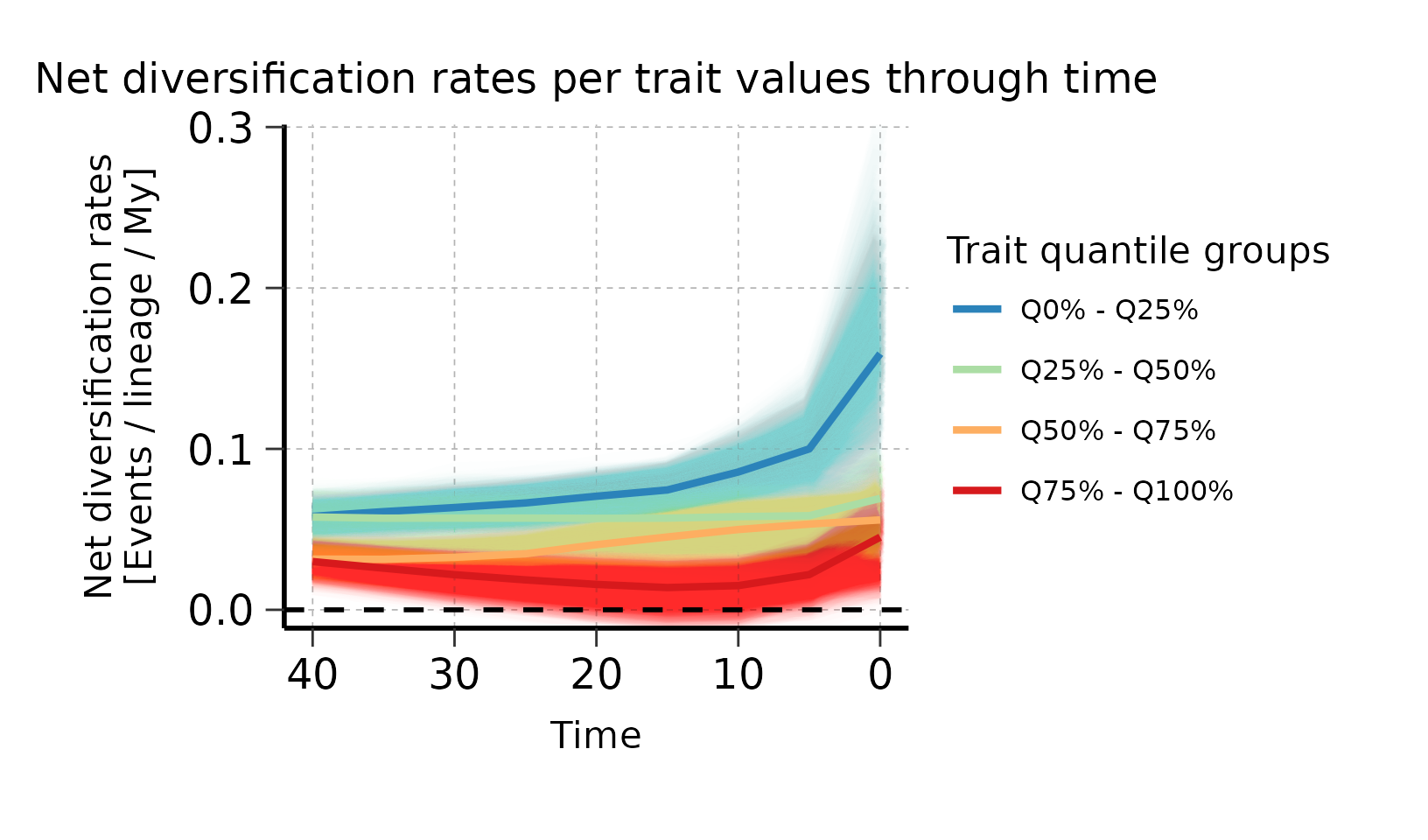

### 4.4/ Plot rates vs. ranges across branches for a given focal time ####

# ?deepSTRAPP::plot_rates_vs_trait_data_for_focal_time()
# ?deepSTRAPP::plot_rates_vs_trait_data_over_time()

# This plot help to visualize differences in rates vs. ranges across all branches
# found at specific time-steps (i.e., 'focal_time').

# Generate ggplot for time = 20 My
plot_rates_vs_trait_data_for_focal_time(
   deepSTRAPP_outputs = Ponerinae_deepSTRAPP_cont_old_calib_0_40,
   focal_time = 20,
   color_scale = color_scale)

# Here we focus on T = 20 My to highlight the correlation detected in the previous steps.
# You can see that ants in the highest trait values (in red) exhibits the lowest rates, at this time-step.
# This plot, alongside other results of deepSTRAPP, supports the Diversification Rate Hypothesis in showing 
# how ant lineages with low trait values (e.g., small size) may have accumulated faster
# than ant lineages with high trait value (e.g., large size), especially between 5 to 25 My.
# Additionally, the plot displays summary statistics for the STRAPP test associated with the data shown:
#   * An observed statistic computed across the mean rates and trait values shown on the plot.
#     Here, rho obs = -0.743, indicating a negative correlation between size and diversification in ponerine ants.
#     This is not the statistic of the STRAPP test itself, which is conducted across all BAMM posterior samples.
#   * The quantile of null statistic distribution at the significant threshold used to define test significance. 
#     The test will be considered significant (i.e., the null hypothesis is rejected)
#     if this value is higher than zero, as shown on the histogram in Section 4.2.
#     Here, Q5% = 0.036, so the test is significant (according to this significance threshold).
#   * The p-value of the associated STRAPP test. Here, p = 0.022.

# Plot rates vs. ranges for all time-steps
plot_rates_vs_trait_data_over_time(
   deepSTRAPP_outputs = Ponerinae_deepSTRAPP_cont_old_calib_0_40,
   color_scale = color_scale)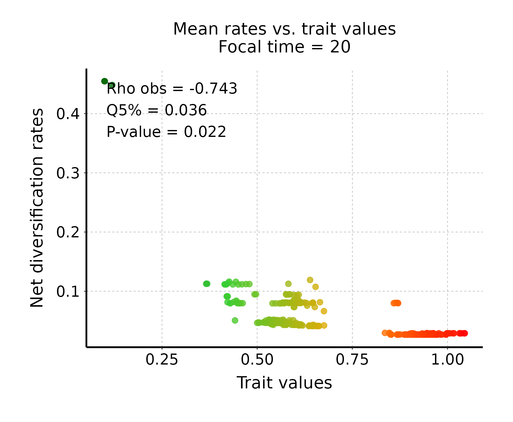

### 4.5/ Plot updated contMap mapping trait evolution for a given 'focal_time' ####

# ?deepSTRAPP::plot_contMap()

## These plots help to visualize the evolution of trait values across the phylogeny, 
## and to focus on tip values at specific time-steps.

# Display the time-steps
Ponerinae_deepSTRAPP_cont_old_calib_0_40$time_steps
#> [1]  0  5 10 15 20 25 30 35 40

# Extract root age
root_age <- max(phytools::nodeHeights(Ponerinae_tree_old_calib)[,2])

## The next plot shows the evolution of trait values across the whole phylogeny (100-0 My).

# Plot initial contMap (t = 0)
contMap_0My <- Ponerinae_deepSTRAPP_cont_old_calib_0_40$updated_trait_data_with_Map_over_time[[1]]
plot_contMap(contMap_0My$contMap,
             color_scale = c("darkgreen", "limegreen", "orange", "red"),
             lwd = 0.7, # Adjust width of branches
             fsize = c(0.1, 1)) # Reduce tip label size
abline(v = root_age - 20, col = "red", lty = 2) # Show where the phylogeny will be cut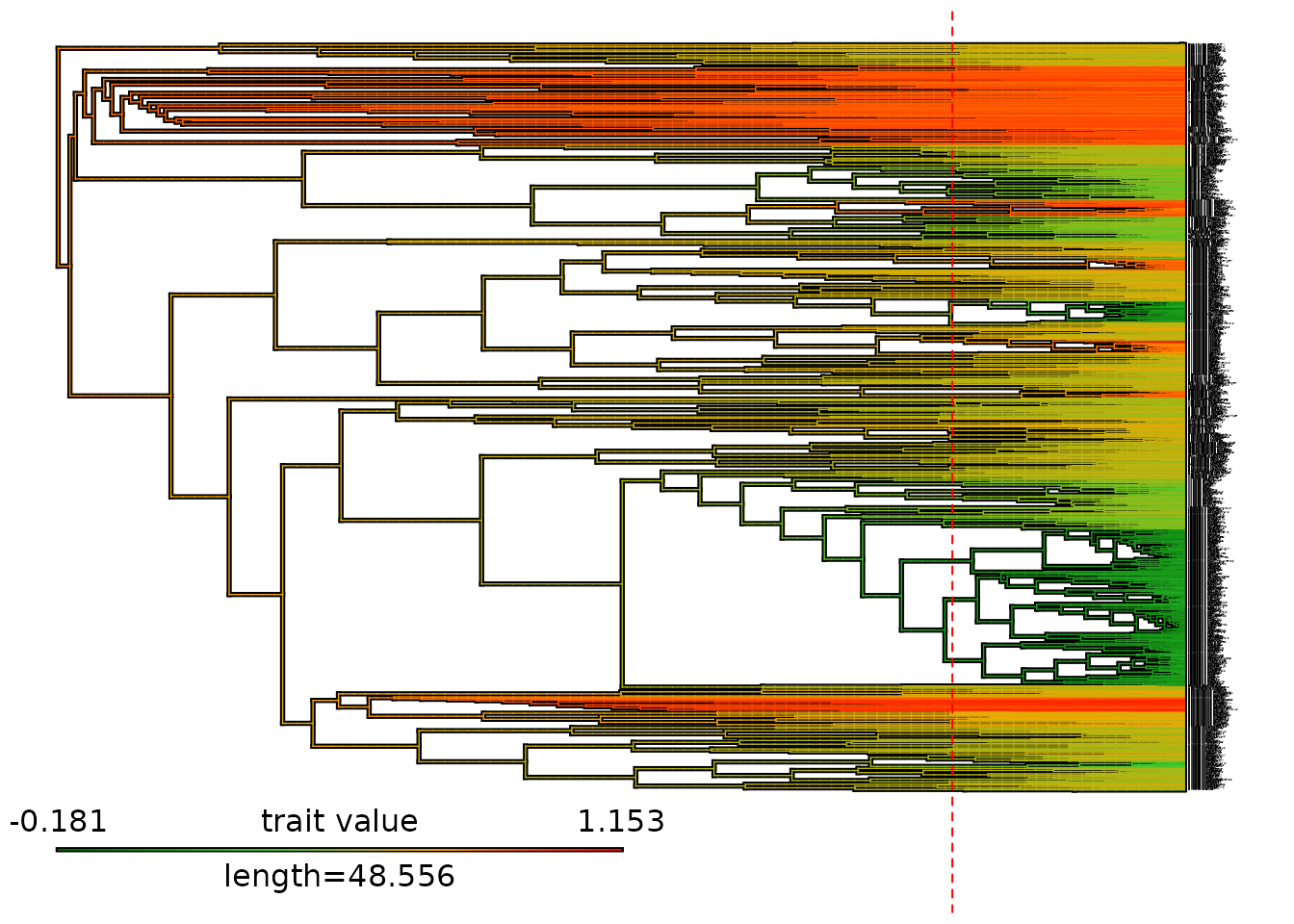


## The next plot shows the evolution of trait values from root to 20Mya (100-20 My).

# Plot updated contMap for time-step n°5 = 20 My
contMap_20My <- Ponerinae_deepSTRAPP_cont_old_calib_0_40$updated_trait_data_with_Map_over_time[[5]]
plot_contMap(contMap_20My$contMap,
             color_scale = c("darkgreen", "limegreen", "orange", "red"),
             lwd = 0.9, # Adjust width of branches
             fsize = c(0.2, 1)) # Reduce tip label size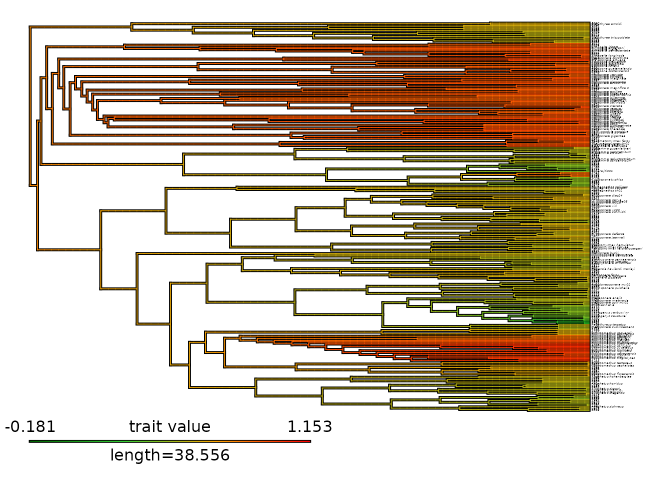

### 4.6/ Plot updated diversification rates and regimes for a given 'focal_time' ####

# ?deepSTRAPP::plot_BAMM_rates()

## These plots help to visualize the evolution of diversification rates across the phylogeny,
## and to focus on tip values at specific time-steps.

# Display the time-steps
Ponerinae_deepSTRAPP_cont_old_calib_0_40$time_steps

# Extract root age
root_age <- max(phytools::nodeHeights(Ponerinae_tree_old_calib)[,2])

## The next plot shows the evolution of net diversification rates across the whole phylogeny (100-0 My).

# Plot diversification rates on initial phylogeny (t = 0)
BAMM_map_0My <- Ponerinae_deepSTRAPP_cont_old_calib_0_40$updated_BAMM_objects_over_time[[1]]
plot_BAMM_rates(BAMM_map_0My, labels = FALSE, par.reset = FALSE)
abline(v = root_age - 20, col = "red", lty = 2) # Show where the phylogeny will be cut
title(main = "BAMM rates for 100-0 My")

## The next plot shows the evolution of net diversification rates from root to 20 Mya (100-20 My).

# Plot diversification rates on updated phylogeny for time-step n°5 = 20 My
BAMM_map_20My <- Ponerinae_deepSTRAPP_cont_old_calib_0_40$updated_BAMM_objects_over_time[[5]]
plot_BAMM_rates(BAMM_map_20My, labels = FALSE,
                colorbreaks = BAMM_map_20My$initial_colorbreaks$net_diversification)
title(main = "BAMM rates for 100-20 My")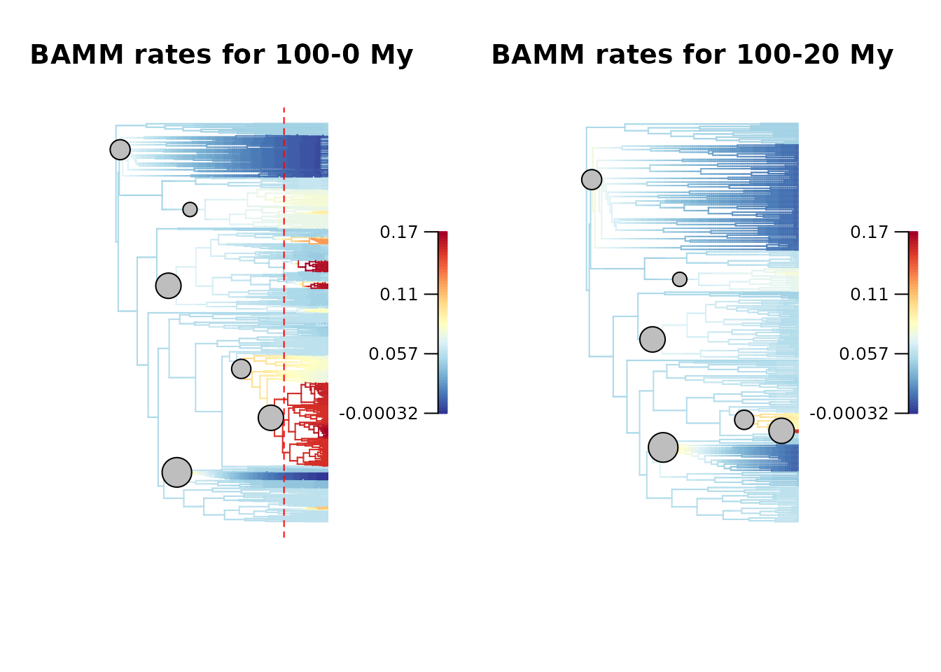

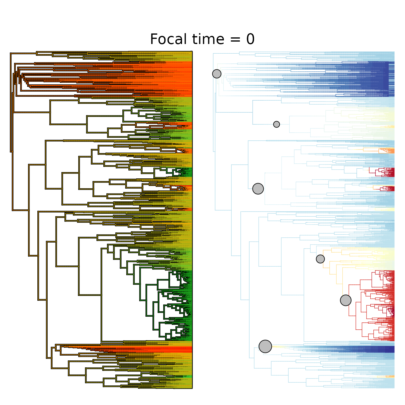
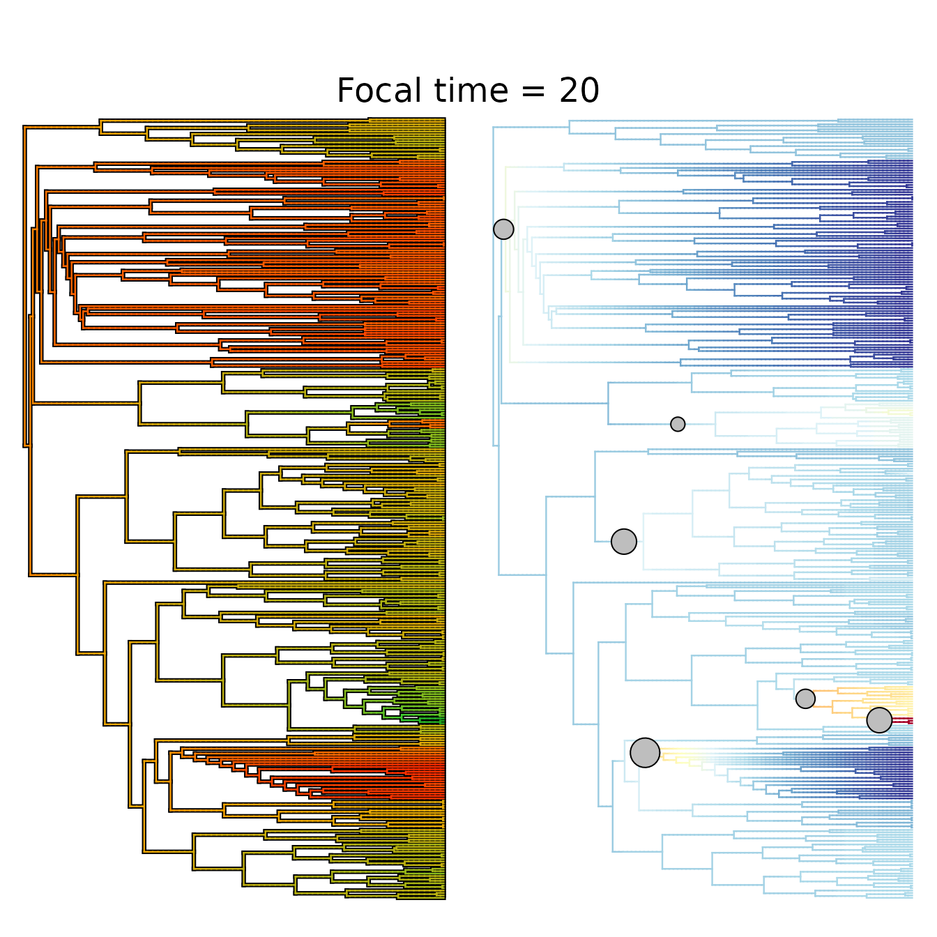
### 4.7/ Plot both trait evolution and diversification rates and regimes updated for a given 'focal_time' ####

# ?deepSTRAPP::plot_traits_vs_rates_on_phylogeny_for_focal_time()

## These plots help to visualize simultaneously the evolution of trait and diversification rates
## across the phylogeny, and to focus on tip values at specific time-steps.

# Display the time-steps
Ponerinae_deepSTRAPP_cont_old_calib_0_40$time_steps

## The next plot shows the evolution of trait values and rates across the whole phylogeny (100-0 My).

# Plot diversification rates on initial phylogeny (t = 0)
plot_traits_vs_rates_on_phylogeny_for_focal_time(
  deepSTRAPP_outputs = Ponerinae_deepSTRAPP_cont_old_calib_0_40,
  focal_time = 0,
  ftype = "off", lwd = 0.7,
  color_scale = c("darkgreen", "limegreen", "orange", "red"),
  labels = FALSE, legend = FALSE,
  par.reset = FALSE)

## The next plot shows the evolution of trait values and rates from root to 20 Mya (100-20 My).

# Plot diversification rates on updated phylogeny for time-step n°5 = 20 My
plot_traits_vs_rates_on_phylogeny_for_focal_time(
  deepSTRAPP_outputs = Ponerinae_deepSTRAPP_cont_old_calib_0_40,
  focal_time = 20, 
  ftype = "off", lwd = 1.2,
  color_scale = c("darkgreen", "limegreen", "orange", "red"),
  labels = FALSE, legend = FALSE,
  par.reset = FALSE)

Maël Doré

2025-10-22