Extract trait data mapped on a phylogeny at a given time in the past

Extracts the most likely trait values found along branches at a specific time in the past (i.e. the focal_time). Optionally, the function can update the mapped phylogeny (contMap or densityMaps) such as branches overlapping the focal_time are shorten to the focal_time, and the trait mapping for the cut off branches are removed by updating the $tree$maps and $tree$mapped.edge elements.

Usage

extract_most_likely_trait_values_for_focal_time(
  contMap = NULL,
  densityMaps = NULL,
  ace = NULL,
  tip_data = NULL,
  trait_data_type,
  focal_time,
  update_map = FALSE,
  keep_tip_labels = TRUE
)

Arguments

contMap

For continuous trait data. Object of class "contMap", typically generated with prepare_trait_data() or phytools::contMap(), that contains a phylogenetic tree and associated continuous trait mapping. The phylogenetic tree must be rooted and fully resolved/dichotomous, but it does not need to be ultrametric (it can includes fossils).

densityMaps

For categorical trait or biogeographic data. List of objects of class "densityMap", typically generated with prepare_trait_data(), that contains a phylogenetic tree and associated posterior probability of being in a given state/range along branches. Each object (i.e., densityMap) corresponds to a state/range. The phylogenetic tree must be rooted and fully resolved/dichotomous, but it does not need to be ultrametric (it can includes fossils).

ace

(Optional) Ancestral Character Estimates (ACE) at the internal nodes. Obtained with prepare_trait_data() as output in the $ace slot.

• For continuous trait data: Named numerical vector typically generated with phytools::fastAnc(), phytools::anc.ML(), or ape::ace(). Names are nodes_ID of the internal nodes. Values are ACE of the trait.

• For categorical trait or biogeographic data: Matrix that record the posterior probabilities of ancestral states/ranges. Rows are internal nodes_ID. Columns are states/ranges. Values are posterior probabilities of each state per node. Needed in all cases to provide accurate estimates of trait values.

tip_data

(Optional) Named vector of tip values of the trait.

• For continuous trait data: Named numerical vector of trait values.

• For categorical trait or biogeographic data: Character string vector of states/ranges Names are nodes_ID of the internal nodes. Needed to provide accurate tip values.

trait_data_type

Character string. Specify the type of trait data. Must be one of "continuous", "categorical", "biogeographic".

focal_time

Integer. The time, in terms of time distance from the present, at which the tree and mapping must be cut. It must be smaller than the root age of the phylogeny.

update_map

Logical. Specify whether the mapped phylogeny (contMap or densityMaps) provided as input should be updated for visualization and returned among the outputs. Default is FALSE. The update consists in cutting off branches and mapping that are younger than the focal_time.

keep_tip_labels

Logical. Specify whether terminal branches with a single descendant tip must retained their initial tip.label on the updated contMap. Default is TRUE. Used only if update_map = TRUE.

Value

By default, the function returns a list with three elements.

• $trait_data A named numerical vector with ML trait values found along branches overlapping the focal_time. Names are the tip.label/tipward node ID.

• $focal_time Integer. The time, in terms of time distance from the present, at which the trait data were extracted.

• $trait_data_type Character string. Define the type of trait data as "continuous", "categorical", or "biogeographic". Used in downstream analyses to select appropriate statistical processing.

If update_map = TRUE, the output is a list with four elements: $trait_data, $focal_time, $trait_data_type, and $contMap or $densityMaps.

For continuous trait data:

• $contMap An object of class "contMap" that contains the updated contMap with branches and mapping that are younger than the focal_time cut off. The function also adds multiple useful sub-elements to the $contMap$tree element.

  • $root_age Integer. Stores the age of the root of the tree.

  • $nodes_ID_df Data.frame with two columns. Provides the conversion from the new_node_ID to the initial_node_ID. Each row is a node.

  • $initial_nodes_ID Vector of character strings. Provides the initial ID of internal nodes. Used to plot internal node IDs as labels with ape::nodelabels().

  • $edges_ID_df Data.frame with two columns. Provides the conversion from the new_edge_ID to the initial_edge_ID. Each row is an edge/branch.

  • $initial_edges_ID Vector of character strings. Provides the initial ID of edges/branches. Used to plot edge/branch IDs as labels with ape::edgelabels().

For categorical trait and biogeographic data:

• $densityMaps A list of objects of class "densityMap" that contains the updated densityMap of each state/range, with branches and mapping that are younger than the focal_time cut off. The function also adds multiple useful sub-elements to the $densityMaps$tree elements.

  • $root_age Integer. Stores the age of the root of the tree.

  • $nodes_ID_df Data.frame with two columns. Provides the conversion from the new_node_ID to the initial_node_ID. Each row is a node.

  • $initial_nodes_ID Vector of character strings. Provides the initial ID of internal nodes. Used to plot internal node IDs as labels with ape::nodelabels().

  • $edges_ID_df Data.frame with two columns. Provides the conversion from the new_edge_ID to the initial_edge_ID. Each row is an edge/branch.

  • $initial_edges_ID Vector of character strings. Provides the initial ID of edges/branches. Used to plot edge/branch IDs as labels with ape::edgelabels().

Details

The mapped phylogeny (contMap or densityMaps) is cut at a specific time in the past (i.e. the focal_time) and the current trait values of the overlapping edges/branches are extracted.

—– Extract trait_data —–

For continuous trait data:

If providing only the contMap trait values at tips and internal nodes will be extracted from the mapping of the contMap leading to a slight discrepancy with the actual tip data and estimated ancestral character values.

True ML trait estimates will be used if tip_data and/or ace are provided as optional inputs. In practice the discrepancy is negligible.

For categorical trait and biogeographic data:

Most likely states/ranges are extracted from the posterior probabilities displayed in the densityMaps. The states/ranges with the highest probability is assigned to each tip and cut branches at focal_time.

True ML states/ranges will be used if tip_data and/or ace are provided as optional inputs. In practice the discrepancy is negligible.

—– Update the contMap/densityMaps —–

To obtain an updated contMap/densityMaps alongside the trait data, set update_map = TRUE. The update consists in cutting off branches and mapping that are younger than the focal_time.

• When a branch with a single descendant tip is cut and keep_tip_labels = TRUE, the leaf left is labeled with the tip.label of the unique descendant tip.

• When a branch with a single descendant tip is cut and keep_tip_labels = FALSE, the leaf left is labeled with the node ID of the unique descendant tip.

• In all cases, when a branch with multiple descendant tips (i.e., a clade) is cut, the leaf left is labeled with the node ID of the MRCA of the cut-off clade.

The mapping in contMap/densityMaps ($tree$maps and $tree$mapped.edge) is updated accordingly by removing mapping associated with the cut off branches.

A specific sub-function (that can be used independently) is called according to the type of trait data:

• For continuous traits: extract_most_likely_trait_values_from_contMap_for_focal_time()

• For categorical traits: extract_most_likely_states_from_densityMaps_for_focal_time()

• For biogeographic ranges: extract_most_likely_ranges_from_densityMaps_for_focal_time()

See also

cut_phylo_for_focal_time() cut_contMap_for_focal_time() cut_densityMaps_for_focal_time()

Associated sub-functions per type of trait data:

extract_most_likely_trait_values_from_contMap_for_focal_time() extract_most_likely_states_from_densityMaps_for_focal_time() extract_most_likely_ranges_from_densityMaps_for_focal_time()

Author

Maël Doré

Examples

# ----- Example 1: Continuous trait ----- #

## Prepare data

# Load eel data from the R package phytools
# Source: Collar et al., 2014; DOI: 10.1038/ncomms6505

library(phytools)
data(eel.tree)
data(eel.data)

# Extract body size
eel_data <- setNames(eel.data$Max_TL_cm,
                     rownames(eel.data))

# Get Ancestral Character Estimates based on a Brownian Motion model
# To obtain values at internal nodes
eel_ACE <- phytools::fastAnc(tree = eel.tree, x = eel_data)

# Run a Stochastic Mapping based on a Brownian Motion model
# to interpolate values along branches and obtain a "contMap" object
eel_contMap <- phytools::contMap(eel.tree, x = eel_data,
                                 res = 100, # Number of time steps
                                 plot = FALSE)

# Set focal time to 50 Mya
focal_time <- 50

## Extract trait data and update contMap for the given focal_time

# Extract from the contMap (values are not exact ML estimates)
eel_cont_50 <- extract_most_likely_trait_values_for_focal_time(
   contMap = eel_contMap,
   trait_data_type = "continuous",
   focal_time = focal_time,
   update_map = TRUE)
#> WARNING: No ancestral character estimates (ace) for internal nodes have been provided. Using values interpolated in the contMap instead.
#> WARNING: No tip data have been provided. Using values interpolated in the contMap instead.
# Extract from tip data and ML estimates of ancestral characters (values are true ML estimates)
eel_cont_50 <- extract_most_likely_trait_values_for_focal_time(
   contMap = eel_contMap,
   ace = eel_ACE, tip_data = eel_data,
   trait_data_type = "continuous",
   focal_time = focal_time,
   update_map = TRUE)
#> Warning: Values in 'tip_data' are not ordered as tip labels in the contMap$tree.
#> They were reordered to follow tip labels.

## Visualize outputs

# Print trait data
eel_cont_50$trait_data
#>    Moringua_edwardsi Kaupichthys_nuchalis                   69 
#>             52.70485             65.25449             71.66003 
#>                   70                   81                   89 
#>             79.15280             76.11928             86.04101 
#>                  101                  103    Serrivomer_sector 
#>             82.04332            100.55349             94.72769 
#>  Paraconger_notialis    Moringua_javanica                  121 
#>             75.04175             95.62468            108.30889 
#>        Albula_vulpes 
#>            105.09029 

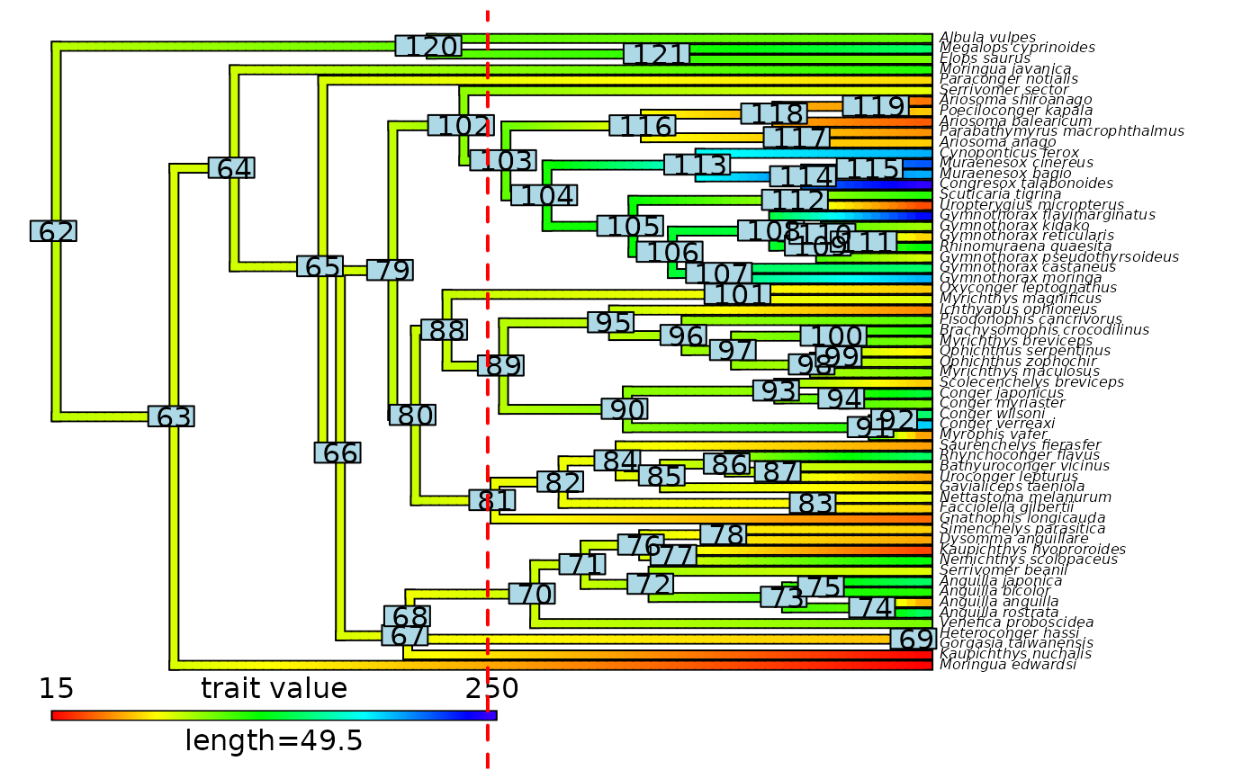
# Plot node labels on initial stochastic map with cut-off
plot(eel_contMap, fsize = c(0.5, 1))
ape::nodelabels()
abline(v = max(phytools::nodeHeights(eel_contMap$tree)[,2]) - focal_time,
       col = "red", lty = 2, lwd = 2)


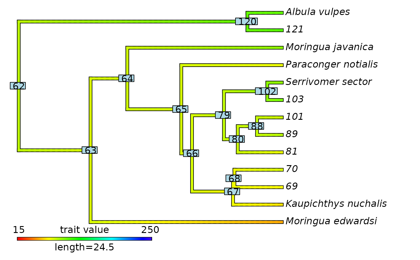
# Plot updated contMap with initial node labels
plot(eel_cont_50$contMap)
ape::nodelabels(text = eel_cont_50$contMap$tree$initial_nodes_ID)



# ----- Example 2: Categorical trait ----- #

## Load categorical trait data mapped on a phylogeny
data(eel_cat_3lvl_data, package = "deepSTRAPP")

# Explore data
str(eel_cat_3lvl_data, 1)
#> List of 6
#>  $ densityMaps       :List of 3
#>  $ trait_data_type   : chr "categorical"
#>  $ simmaps           :Class "multiPhylo"
#> List of 100
#>  $ ace               : num [1:60, 1:3] 0.26 0.3 0.39 0.43 0.43 0.44 0.43 0 0.47 0.49 ...
#>   ..- attr(*, "dimnames")=List of 2
#>  $ best_model_fit    :List of 4
#>   ..- attr(*, "class")= chr [1:2] "gfit" "list"
#>  $ model_selection_df:'data.frame':	5 obs. of  6 variables:
eel_cat_3lvl_data$densityMaps # Three density maps: one per state
#> $Density_map_bite
#> Object of class "densityMap" containing:
#> 
#> (1) A phylogenetic tree with 61 tips and 60 internal nodes.
#> 
#> (2) The mapped posterior density of a discrete binary character
#>     with states (Not bite, bite).
#> 
#> 
#> $Density_map_kiss
#> Object of class "densityMap" containing:
#> 
#> (1) A phylogenetic tree with 61 tips and 60 internal nodes.
#> 
#> (2) The mapped posterior density of a discrete binary character
#>     with states (Not kiss, kiss).
#> 
#> 
#> $Density_map_suction
#> Object of class "densityMap" containing:
#> 
#> (1) A phylogenetic tree with 61 tips and 60 internal nodes.
#> 
#> (2) The mapped posterior density of a discrete binary character
#>     with states (Not suction, suction).
#> 
#> 

# Set focal time to 10 Mya
focal_time <- 10

## Extract trait data and update densityMaps for the given focal_time

# Extract from the densityMaps
eel_cat_3lvl_data_10My <- extract_most_likely_trait_values_for_focal_time(
   densityMaps = eel_cat_3lvl_data$densityMaps,
   trait_data_type = "categorical",
   focal_time = focal_time,
   update_map = TRUE)
#> WARNING: No ancestral character estimates (ace) for internal nodes have been provided. Using most likely states extracted from the densityMaps instead.
#> WARNING: No tip data have been provided. Using states extracted from the densityMaps instead.

## Print trait data
str(eel_cat_3lvl_data_10My, 1)
#> List of 4
#>  $ trait_data     : Named chr [1:52] "bite" "bite" "suction" "bite" ...
#>   ..- attr(*, "names")= chr [1:52] "Moringua_edwardsi" "Kaupichthys_nuchalis" "69" "Venefica_proboscidea" ...
#>  $ focal_time     : num 10
#>  $ trait_data_type: chr "categorical"
#>  $ densityMaps    :List of 3
eel_cat_3lvl_data_10My$trait_data
#>             Moringua_edwardsi          Kaupichthys_nuchalis 
#>                        "bite"                        "bite" 
#>                            69          Venefica_proboscidea 
#>                     "suction"                        "bite" 
#>                            74              Anguilla_bicolor 
#>                     "suction"                     "suction" 
#>             Anguilla_japonica             Serrivomer_beanii 
#>                     "suction"                        "bite" 
#>        Nemichthys_scolopaceus      Kaupichthys_hyoproroides 
#>                        "bite"                        "bite" 
#>            Dysomma_anguillare        Simenchelys_parasitica 
#>                        "kiss"                        "kiss" 
#>         Gnathophis_longicauda         Facciolella_gilbertii 
#>                     "suction"                        "bite" 
#>          Nettastoma_melanurum          Gavialiceps_taeniola 
#>                        "bite"                        "bite" 
#>            Uroconger_lepturus        Bathyuroconger_vicinus 
#>                     "suction"                        "bite" 
#>          Rhynchoconger_flavus        Saurenchelys_fierasfer 
#>                        "kiss"                        "kiss" 
#>                            91                            94 
#>                     "suction"                     "suction" 
#>      Scolecenchelys_breviceps          Myrichthys_maculosus 
#>                     "suction"                     "suction" 
#>                            99          Myrichthys_breviceps 
#>                     "suction"                     "suction" 
#>   Brachysomophis_crocodilinus      Pisodonophis_cancrivorus 
#>                     "suction"                        "bite" 
#>          Ichthyapus_ophioneus         Myrichthys_magnificus 
#>                        "kiss"                     "suction" 
#>        Oxyconger_leptognathus           Gymnothorax_moringa 
#>                        "bite"                        "bite" 
#>         Gymnothorax_castaneus Gymnothorax_pseudothyrsoideus 
#>                        "bite"                        "kiss" 
#>                           111            Gymnothorax_kidako 
#>                        "kiss"                        "kiss" 
#>   Gymnothorax_flavimarginatus      Uropterygius_micropterus 
#>                        "kiss"                        "kiss" 
#>            Scuticaria_tigrina        Congresox_talabonoides 
#>                        "kiss"                        "kiss" 
#>                           115            Cynoponticus_ferox 
#>                        "bite"                        "kiss" 
#>                Ariosoma_anago Parabathymyrus_macrophthalmus 
#>                        "kiss"                     "suction" 
#>           Ariosoma_balearicum                           119 
#>                        "kiss"                     "suction" 
#>             Serrivomer_sector           Paraconger_notialis 
#>                        "bite"                     "suction" 
#>             Moringua_javanica                  Elops_saurus 
#>                        "bite"                     "suction" 
#>          Megalops_cyprinoides                 Albula_vulpes 
#>                     "suction"                        "kiss" 

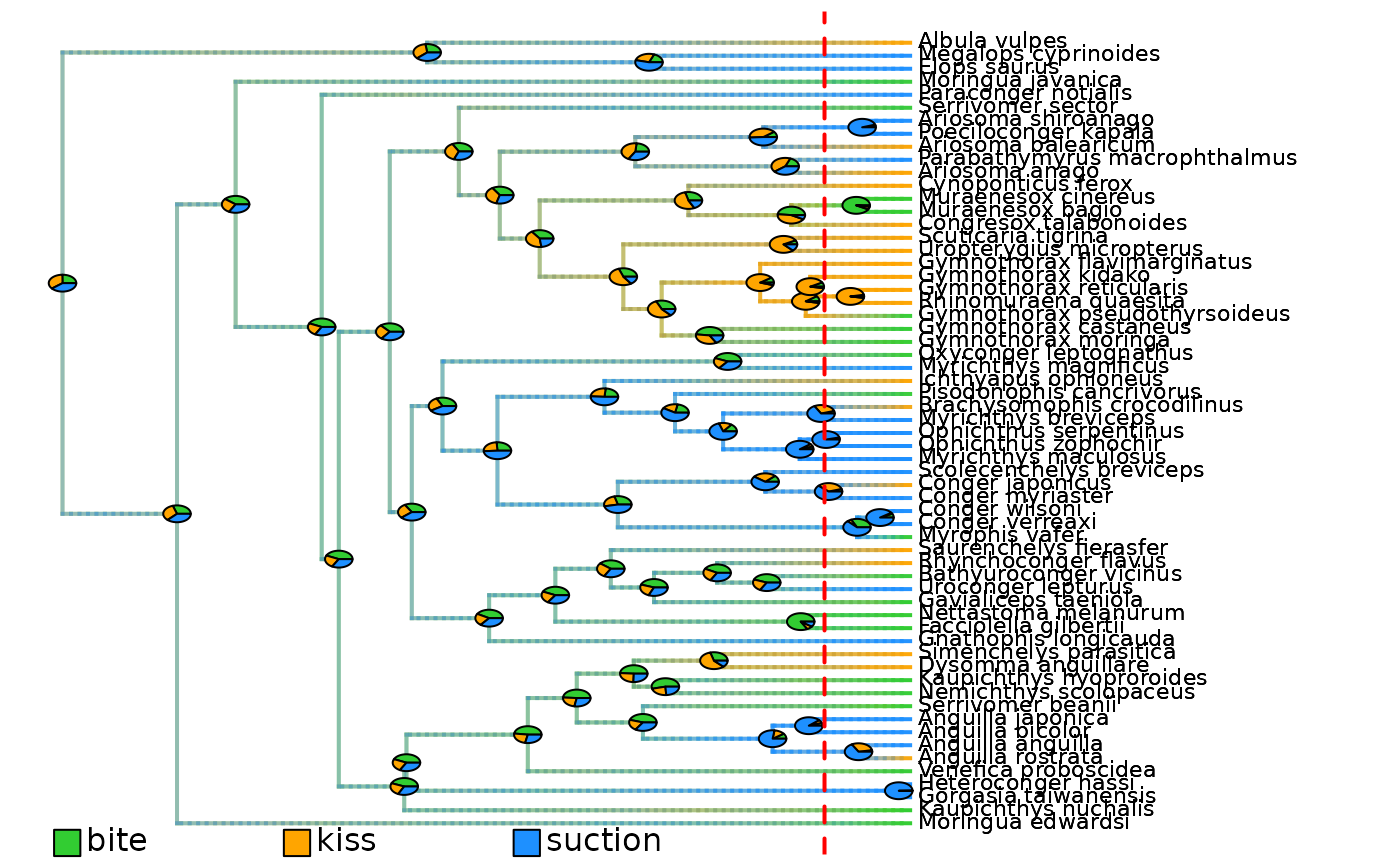
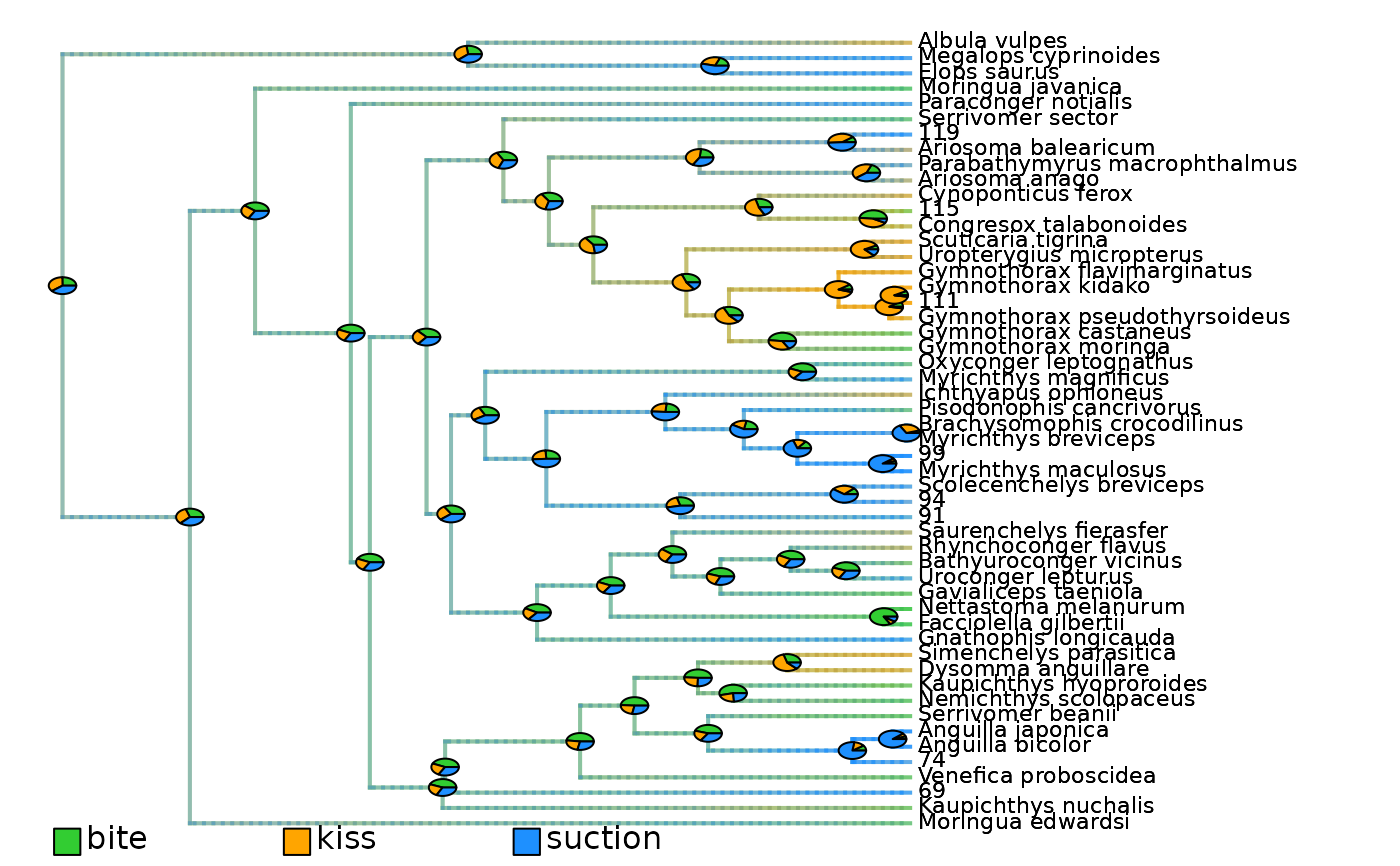
## Plot density maps as overlay of all state posterior probabilities

# Plot initial density maps with ACE pies
plot_densityMaps_overlay(densityMaps = eel_cat_3lvl_data$densityMaps)
abline(v = max(phytools::nodeHeights(eel_cat_3lvl_data$densityMaps[[1]]$tree)[,2]) - focal_time,
       col = "red", lty = 2, lwd = 2)


# Plot updated densityMaps with ACE pies
plot_densityMaps_overlay(eel_cat_3lvl_data_10My$densityMaps)



# ----- Example 3: Biogeographic ranges ----- #

## Load biogeographic range data mapped on a phylogeny
data(eel_biogeo_data, package = "deepSTRAPP")

# Explore data
str(eel_biogeo_data, 1)
#> List of 9
#>  $ densityMaps           :List of 2
#>  $ densityMaps_all_ranges:List of 3
#>  $ trait_data_type       : chr "biogeographic"
#>  $ ace                   : num [1:60, 1:2] 0.361 0.524 0.623 0.334 0.47 ...
#>   ..- attr(*, "dimnames")=List of 2
#>  $ ace_all_ranges        : num [1:60, 1:3] 0.174 0.373 0.53 0.244 0.411 ...
#>   ..- attr(*, "dimnames")=List of 2
#>  $ BSM_output            :List of 2
#>  $ simmaps               :Class "multiPhylo"
#> List of 100
#>  $ best_model_fit        :List of 13
#>   ..- attr(*, "class")= chr "calc_loglike_sp_results"
#>  $ model_selection_df    :'data.frame':	6 obs. of  8 variables:
eel_biogeo_data$densityMaps # Two density maps: one per unique area: A, B.
#> $Density_map_A
#> Object of class "densityMap" containing:
#> 
#> (1) A phylogenetic tree with 61 tips and 60 internal nodes.
#> 
#> (2) The mapped posterior density of a discrete binary character
#>     with states (Not A, A).
#> 
#> 
#> $Density_map_B
#> Object of class "densityMap" containing:
#> 
#> (1) A phylogenetic tree with 61 tips and 60 internal nodes.
#> 
#> (2) The mapped posterior density of a discrete binary character
#>     with states (Not B, B).
#> 
#> 
eel_biogeo_data$densityMaps_all_ranges # Three density maps: one per range: A, B, and AB.
#> $Density_map_A
#> Object of class "densityMap" containing:
#> 
#> (1) A phylogenetic tree with 61 tips and 60 internal nodes.
#> 
#> (2) The mapped posterior density of a discrete binary character
#>     with states (Not A, A).
#> 
#> 
#> $Density_map_B
#> Object of class "densityMap" containing:
#> 
#> (1) A phylogenetic tree with 61 tips and 60 internal nodes.
#> 
#> (2) The mapped posterior density of a discrete binary character
#>     with states (Not B, B).
#> 
#> 
#> $Density_map_AB
#> Object of class "densityMap" containing:
#> 
#> (1) A phylogenetic tree with 61 tips and 60 internal nodes.
#> 
#> (2) The mapped posterior density of a discrete binary character
#>     with states (Not AB, AB).
#> 
#> 

# Set focal time to 10 Mya
focal_time <- 10

## Extract trait data and update densityMaps for the given focal_time

# Extract from the densityMaps
eel_biogeo_data_10My <- extract_most_likely_trait_values_for_focal_time(
   densityMaps = eel_biogeo_data$densityMaps,
   # ace = eel_biogeo_data$ace,
   trait_data_type = "biogeographic",
   focal_time = focal_time,
   update_map = TRUE)
#> WARNING: No ancestral character estimates (ace) for internal nodes have been provided. Using most likely ranges extracted from the densityMaps instead.
#> WARNING: No tip data have been provided. Using ranges extracted from the densityMaps instead.

## Print trait data
str(eel_biogeo_data_10My, 1)
#> List of 4
#>  $ trait_data     : Named chr [1:52] "B" "B" "B" "A" ...
#>   ..- attr(*, "names")= chr [1:52] "Moringua_edwardsi" "Kaupichthys_nuchalis" "69" "Venefica_proboscidea" ...
#>  $ focal_time     : num 10
#>  $ trait_data_type: chr "biogeographic"
#>  $ densityMaps    :List of 2
eel_biogeo_data_10My$trait_data
#>             Moringua_edwardsi          Kaupichthys_nuchalis 
#>                           "B"                           "B" 
#>                            69          Venefica_proboscidea 
#>                           "B"                           "A" 
#>                            74              Anguilla_bicolor 
#>                           "B"                           "B" 
#>             Anguilla_japonica             Serrivomer_beanii 
#>                           "B"                           "A" 
#>        Nemichthys_scolopaceus      Kaupichthys_hyoproroides 
#>                           "A"                           "A" 
#>            Dysomma_anguillare        Simenchelys_parasitica 
#>                           "A"                           "A" 
#>         Gnathophis_longicauda         Facciolella_gilbertii 
#>                           "B"                           "A" 
#>          Nettastoma_melanurum          Gavialiceps_taeniola 
#>                           "A"                           "A" 
#>            Uroconger_lepturus        Bathyuroconger_vicinus 
#>                           "A"                           "A" 
#>          Rhynchoconger_flavus        Saurenchelys_fierasfer 
#>                           "A"                           "A" 
#>                            91                            94 
#>                           "B"                           "B" 
#>      Scolecenchelys_breviceps          Myrichthys_maculosus 
#>                           "B"                           "B" 
#>                            99          Myrichthys_breviceps 
#>                           "B"                           "B" 
#>   Brachysomophis_crocodilinus      Pisodonophis_cancrivorus 
#>                           "A"                           "A" 
#>          Ichthyapus_ophioneus         Myrichthys_magnificus 
#>                           "A"                           "B" 
#>        Oxyconger_leptognathus           Gymnothorax_moringa 
#>                           "A"                           "A" 
#>         Gymnothorax_castaneus Gymnothorax_pseudothyrsoideus 
#>                           "A"                           "A" 
#>                           111            Gymnothorax_kidako 
#>                           "A"                           "A" 
#>   Gymnothorax_flavimarginatus      Uropterygius_micropterus 
#>                           "A"                           "A" 
#>            Scuticaria_tigrina        Congresox_talabonoides 
#>                           "A"                           "A" 
#>                           115            Cynoponticus_ferox 
#>                           "A"                           "A" 
#>                Ariosoma_anago Parabathymyrus_macrophthalmus 
#>                           "B"                           "B" 
#>           Ariosoma_balearicum                           119 
#>                           "B"                           "B" 
#>             Serrivomer_sector           Paraconger_notialis 
#>                           "A"                           "B" 
#>             Moringua_javanica                  Elops_saurus 
#>                           "A"                           "B" 
#>          Megalops_cyprinoides                 Albula_vulpes 
#>                           "B"                           "B" 

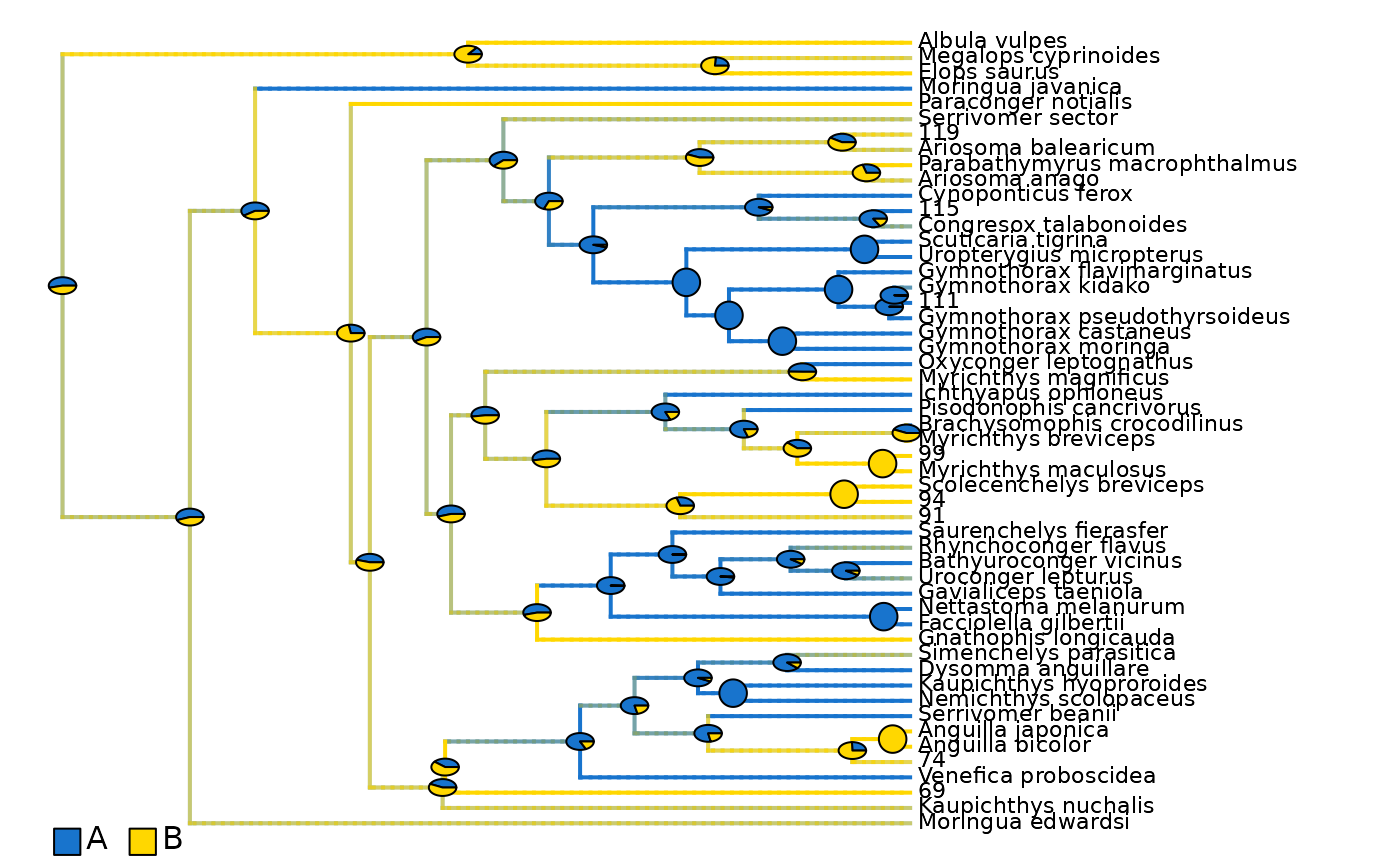
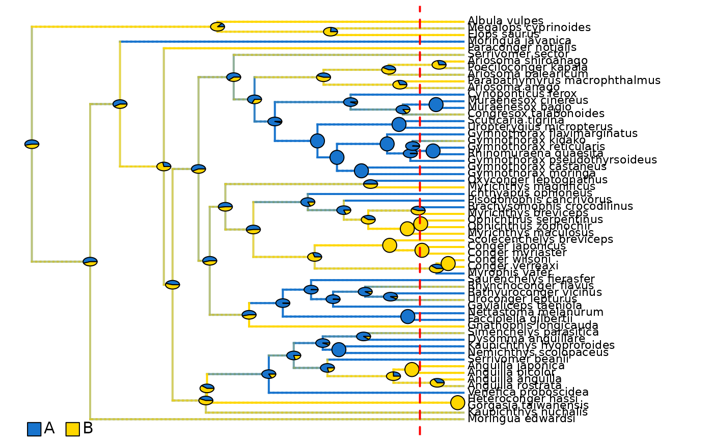
## Plot density maps as overlay of all range posterior probabilities

# Plot initial density maps with ACE pies
plot_densityMaps_overlay(densityMaps = eel_biogeo_data$densityMaps)
abline(v = max(phytools::nodeHeights(eel_biogeo_data$densityMaps[[1]]$tree)[,2]) - focal_time,
       col = "red", lty = 2, lwd = 2)


# Plot updated densityMaps with ACE pies
plot_densityMaps_overlay(eel_biogeo_data_10My$densityMaps)